plotting quantified data
[1]:
# to be able to read unit attributes following the CF conventions
import cf_xarray.units  # noqa: F401  # must be imported before pint_xarray
import xarray as xr

import pint_xarray  # noqa: F401
from pint_xarray import unit_registry as ureg

xr.set_options(display_expand_data=False)
[1]:
<xarray.core.options.set_options at 0x74e53b0e27b0>
load the data
[2]:
ds = xr.tutorial.open_dataset("air_temperature")
data = ds.air
data
[2]:
<xarray.DataArray 'air' (time: 2920, lat: 25, lon: 53)> Size: 31MB
[3869000 values with dtype=float64]
Coordinates:
  * time     (time) datetime64[ns] 23kB 2013-01-01 ... 2014-12-31T18:00:00
  * lat      (lat) float32 100B 75.0 72.5 70.0 67.5 65.0 ... 22.5 20.0 17.5 15.0
  * lon      (lon) float32 212B 200.0 202.5 205.0 207.5 ... 325.0 327.5 330.0
Attributes:
    long_name:     4xDaily Air temperature at sigma level 995
    units:         degK
    precision:     2
    GRIB_id:       11
    GRIB_name:     TMP
    var_desc:      Air temperature
    dataset:       NMC Reanalysis
    level_desc:    Surface
    statistic:     Individual Obs
    parent_stat:   Other
actual_range: [185.16 322.1 ]quantify the data
Note: this example uses the data provided by the xarray.tutorial functions. As such, the units attributes follow the CF conventions, which pint does not understand by default. To still be able to read them we are using the registry provided by cf-xarray.
[3]:
quantified = data.pint.quantify()
quantified
[3]:
<xarray.DataArray 'air' (time: 2920, lat: 25, lon: 53)> Size: 31MB
[K] 241.2 242.5 243.5 244.0 244.1 243.9 ... 297.9 297.4 297.2 296.5 296.2 295.7
Coordinates:
  * time     (time) datetime64[ns] 23kB 2013-01-01 ... 2014-12-31T18:00:00
  * lat      (lat) float32 100B [degrees_north] 75.0 72.5 70.0 ... 17.5 15.0
  * lon      (lon) float32 212B [degrees_east] 200.0 202.5 205.0 ... 327.5 330.0
Indexes:
    lat      PintIndex(PandasIndex, units={'lat': 'degrees_north'})
    lon      PintIndex(PandasIndex, units={'lon': 'degrees_east'})
Attributes:
    long_name:     4xDaily Air temperature at sigma level 995
    precision:     2
    GRIB_id:       11
    GRIB_name:     TMP
    var_desc:      Air temperature
    dataset:       NMC Reanalysis
    level_desc:    Surface
    statistic:     Individual Obs
    parent_stat:   Other
actual_range: [185.16 322.1 ]work with the data
[4]:
monthly_means = quantified.pint.to("degC").sel(time="2013").groupby("time.month").mean()
monthly_means
[4]:
<xarray.DataArray 'air' (month: 12, lat: 25, lon: 53)> Size: 127kB
[°C] -28.68 -28.49 -28.48 -28.67 -28.99 -29.32 ... 24.73 24.77 24.35 24.26 24.22
Coordinates:
  * month    (month) int64 96B 1 2 3 4 5 6 7 8 9 10 11 12
  * lat      (lat) float32 100B [degrees_north] 75.0 72.5 70.0 ... 17.5 15.0
  * lon      (lon) float32 212B [degrees_east] 200.0 202.5 205.0 ... 327.5 330.0
Indexes:
    lat      PintIndex(PandasIndex, units={'lat': 'degrees_north'})
    lon      PintIndex(PandasIndex, units={'lon': 'degrees_east'})
Attributes:
    long_name:     4xDaily Air temperature at sigma level 995
    precision:     2
    GRIB_id:       11
    GRIB_name:     TMP
    var_desc:      Air temperature
    dataset:       NMC Reanalysis
    level_desc:    Surface
    statistic:     Individual Obs
    parent_stat:   Other
actual_range: [185.16 322.1 ]Most operations will preserve the units but there are some which will drop them (see the duck array integration status page). To work around that there are unit-aware versions on the .pint accessor. For example, to select data use .pint.sel instead of .sel:
[5]:
monthly_means.sel(
    lat=ureg.Quantity(4350, "angular_minute"),
    lon=ureg.Quantity(12000, "angular_minute"),
)
[5]:
<xarray.DataArray 'air' (month: 12)> Size: 96B
[°C] -26.08 -31.22 -22.49 -15.6 -5.43 ... 0.4102 -0.1338 -3.855 -14.51 -21.41
Coordinates:
  * month    (month) int64 96B 1 2 3 4 5 6 7 8 9 10 11 12
    lat      float32 4B [degrees_north] 72.5
    lon      float32 4B [degrees_east] 200.0
Attributes:
    long_name:     4xDaily Air temperature at sigma level 995
    precision:     2
    GRIB_id:       11
    GRIB_name:     TMP
    var_desc:      Air temperature
    dataset:       NMC Reanalysis
    level_desc:    Surface
    statistic:     Individual Obs
    parent_stat:   Other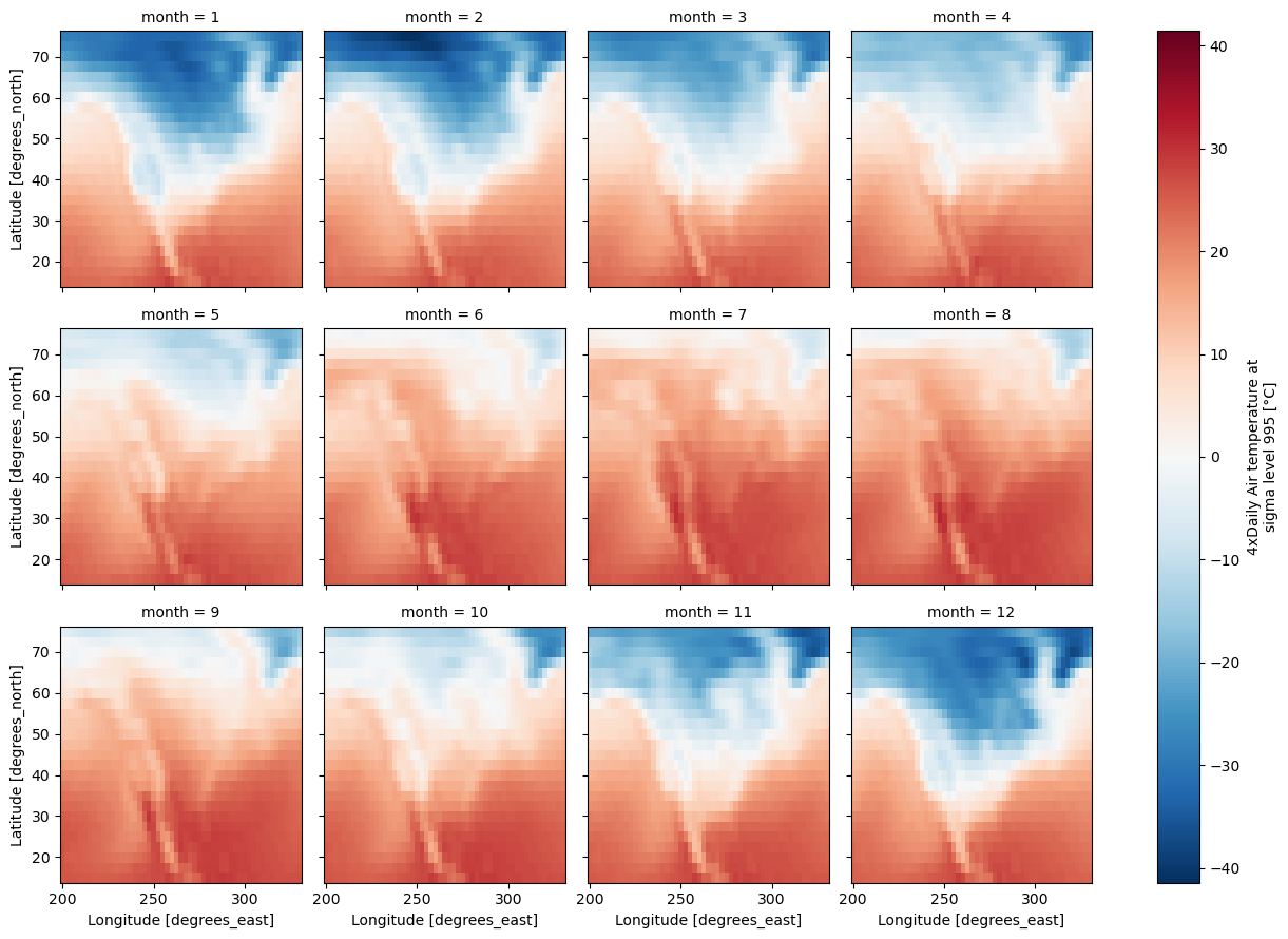
actual_range: [185.16 322.1 ]plot
xarray’s plotting functions will cast the data to numpy.ndarray, so we need to “dequantify” first.
[6]:
monthly_means.pint.dequantify(format="~P").plot.imshow(col="month", col_wrap=4)
[6]:
<xarray.plot.facetgrid.FacetGrid at 0x74e539e48830>